Learning by Playing – Solving Sparse Reward Tasks from Scratch

Link to the blog post
Interesting link from unity

I hereby again recall that this work is not mine, but the one of:
Martin Riedmiller, Roland Hafner, Thomas Lampe, Michael Neunert, Jonas Degrave, Tom Van de Wiele, Volodymyr Mnih, Nicolas Heess and Jost Tobias Springenberg
I simply try to make a complete summary, that is easier to quickly read than the original paper. Thanks for the authors for contributing to science in such an incredible manner!

 Abstract :
Scheduled Auxiliary Control (SACX):
a new learning paradigm in the context of RL
SAC-X enables:

• learning of complex behaviors
• From scratch
• Multiple sparse reward signals

agent is equipped with a set of general auxiliary tasks, that it attempts to learn simultaneously via off-policy RL
key idea: active (learned) scheduling and execution of auxiliary policies allows the agent to efficiently explore its environment  -> excel at sparse reward RL (demonstration video)

Action like “placing a book in a box” difficult:
The agent has to discover a long sequence of “correct” actions in order to find a configuration of the environment that yields the sparse reward

List of techniques developed to answer the problem:

• shaping rewards 
• curriculum learning 
• transfer of learned policies from simulation to reality
• learning from demonstrations 
• learning with model guidance
• inverse RL 

Every time: – need of prior knowledge that is specific to the task.
– Bias the control policy in a direction.

-> goal: develop methods that support the agent during learning but preserve the ability of the agent to learn from sparse rewards.
reduce the specific prior task knowledge that is required to cope with sparse rewards
-> SACX. Principles:

1. Every (s, a) paired with a reward vector of externally provided + internally auxiliary reward
2. The reward vector is composed of fixed particular policy (called intention)
3. High-level scheduler which selects and executes the individual intentions with the goal of improving performance of the agent on the external tasks
4. Learning is performed off-policy (and asynchronously from policy execution) and the experience between intentions is shared – to use information effectively.

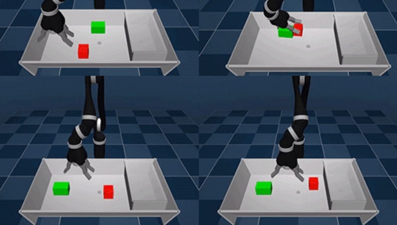
Here robotic experiments on stacking objects and cleaning the table, but this can be extended to other domains.

Auxiliary rewards use the mastery of the agent to control its own sensory observations (e.g. images, proprioception, haptic sensors), and easily implementable (at sensor level (touch or not), or small computation needed (object moved)).

Work on auxiliary tasks:
Sutton & al (2011): general value functions are learned for a large collection of pseudo-rewards corresponding to different goals extracted from the sensorimotor stream.
-> extended to Deep RL in work on Universal Value Function Approximators (UVFA)
Connection to learning to predict the future via “successor” representations or forecasts

Those approaches do not utilize the learned sub-policies to drive exploration for an external “common” goal and typically assume independence between different policies and value functions.

Similar to UVFA, Hindsight Experience Replay, proposed to generate many tasks for a reinforcement learning agent by randomly sampling goals along previously experienced trajectories.

Our approach can be understood as an extension of HER to semantically grounded, and scheduled, goals.

“A related strand of research has considered learning a shared representation for multiple RL tasks”

Closest to this paper are:

• Deep Reinforcement Learning with the UNREAL agent
• Actor Critic agents for navigation
• The Intentional Unintentional Agent

which consider using auxiliary tasks to provide additional learning signals – and additional exploration by following random sensory goals

Here, auxiliary tasks are used by switching between them throughout individual episodes (to achieve exploration for the main task and scheduling the learning and execution of different auxiliary tasks can be understood from the perspective of “teaching” a set of increasingly more complicated problems (fixed number of problems and learn a teaching policy online).

Intrinsic motivation (GRAIL) typically consider internal measures such as learning progress to define rewards, rather than auxiliary tasks that are grounded in physical reality.

• s ∈ R^S be the state 
• MDP M
• a ∈ R^A
• p(s_{t+1}|s_t, a_t)
• π_θ(a|s), policy with parameters θ. 
• scalar reward r_M(s_t, a_t). 
• p(s) initial state distribution

Goal: maximizing the sum of discounted rewards:
\mathbb{E}_{\pi}\left[R\left(\tau_{0: \infty}\right)\right]=\mathbb{E}_{\pi}\left[\sum_{t=0}^{\infty} \gamma^{t} r\left(\mathbf{s}_{t}, \mathbf{a}_{t}\right) a_{t} \sim \pi\left(\cdot | \mathbf{s}_{t}\right), \mathbf{s}_{t+1} \sim p\left(\cdot | \mathbf{s}_{t}, \mathbf{a}_{t}\right), \mathbf{s}_{0} \sim p(\mathbf{s})\right]

Use the short notation to refer to the trajectory starting in state t

Here: Sparse reward problem = finding π∗ in M with a reward function that is characterized by an ’ε region’ in state space:

r_{\mathcal{M}}(\mathbf{s}, \mathbf{a})=\left\{\begin{array}{ll}{\delta_{\mathbf{s}_{g}}(\mathbf{s})} & {\text { if } d\left(\mathbf{s}, \mathbf{s}_{g}\right) \leq \epsilon} \\ {0} & {\text { else }}\end{array}\right.here we will choose the most extreme case where  is small, and we set \delta_{\mathbf{s}_{g}} = 1.

“The auxiliary tasks we define follow a general principle: they encourage the agent to explore its sensor space. For example, activating a touch sensor in its fingers, sensing a force in its wrist, maximising a joint angle in its proprioceptive sensors or forcing a movement of an object in its visual camera sensors. Each task is associated with a simple reward of one if the goal is achieved, and zero otherwise.” (from the blog post)

Formally, let A = {A1,…,AK} denote the set of auxiliary MDPs. These MDPs share the state, observation and action space as well as the transition dynamics with the main task M, but have separate auxiliary reward functions rA1(s,a),…,rAK(s,a). We assume knowledge of how to compute auxiliary rewards and assume we can evaluate them at any state action pair.
\pi_{\boldsymbol{\theta}}(\mathbf{a} | \mathbf{s}, \mathcal{T})= Intention’s policy
\mathbb{E}_{\pi_{\boldsymbol{\theta}}(\mathbf{a} | \mathbf{s}, \mathcal{T})}\left[R_{\mathcal{T}}\left(\tau_{t: \infty}\right)\right]=\mathbb{E}_{\pi_{\boldsymbol{\theta}}(\mathbf{a} | \mathbf{s}, \mathcal{T})}\left[\sum_{t=0}^{\infty} \gamma^{t} r_{\mathcal{T}}\left(\mathbf{s}_{t}, \mathbf{a}_{t}\right)\right]= it’s return

Learning objective : Our goal for learning is to both:

1. train all auxiliary intentions policies and the main task policy to achieve their respective goals
2. utilize all intentions for fast exploration in the main sparse-reward MDP M

We accomplish this by defining a hierarchical objective for policy training that decomposes into two parts:

“Our agent can then decide by itself about its current ‘intention’, i.e. which goal to pursue next. This might be an auxiliary task or an externally defined target task.”
Intention is the agent willing to pursue an (auxiliary or not) task

Joint policy improvement objective for all intentions. Action value function Q_{\mathcal{T}}\left(\mathbf{s}_{t}, \mathbf{a}_{t}\right):
Q_{\mathcal{T}}\left(\mathbf{s}_{t}, \mathbf{a}_{t}\right)=r_{\mathcal{T}}\left(\mathbf{s}_{t}, \mathbf{a}_{t}\right)+\gamma \mathbb{E}_{\pi_{\mathcal{T}}}\left[R_{\mathcal{T}}\left(\tau_{t+1: \infty}\right)\right]

The goal is then to find argmax_θ, for
\begin{aligned} \mathcal{L}(\boldsymbol{\theta}) &=\mathcal{L}(\boldsymbol{\theta} ; \mathcal{M})+\sum_{k=1}^{|A|} \mathcal{L}\left(\boldsymbol{\theta} ; \mathcal{A}_{k}\right) \\ \text { with } \mathcal{L}(\boldsymbol{\theta} ; \mathcal{T}) &=\sum_{\boldsymbol{B} \in \mathcal{Y}} \underset{p(s | \boldsymbol{\zeta})}{\mathbb{E}}\left[Q_{\mathcal{T}}(\mathbf{s}, \mathbf{a})\left|\mathbf{a} \sim \pi_{\boldsymbol{\theta}}(\cdot | \mathbf{s}, \mathcal{T})\right]\right.\end{aligned}

Two comments:
The first term is externally provided loss and the others (in sum) are the internally auxiliary one, I think
Here the loss is common to all the intention, touch mechanism gets penalized for view loss ?

“That is, we optimize each intention to select the optimal action for its task, obtained by following any other policy π(a|s,B) with B∈ T = A∪ {M} (the task which we aimed to solve before). We note that this change is a subtle,yet important, departure from a multi-task RL formulation”

Training policies together (on states sampled according to the state visitation distribution of each possible task), gives policies that are “compatible”.
-> crucial to safely combine the learned intentions

ξ: the period at which the scheduler can switch between tasks

T_{0:H-1} = {T_0, ..., T_{H-1}} the H scheduling choices.
The return is then defined by:

\begin{aligned} R_{\mathcal{M}}\left(\mathcal{T}_{0: H-1}\right) &=\sum_{h=0}^{H} \sum_{t=h \xi}^{(h+1) \xi-1} \gamma^{t} r_{\mathcal{M}}\left(\mathbf{s}_{t}, \mathbf{a}_{t}\right) \\ \text { where } \mathbf{a}_{t} & \sim \pi_{\boldsymbol{\theta}}\left(\cdot | \mathbf{s}_{t}, \mathcal{T}_{h}\right) \end{aligned}

Now with P_{\mathcal{S}}\left(\mathcal{T} | \mathcal{T}_{0: h-1}\right) the scheduling policy, the probability of an action a_t is:
\pi_{\mathcal{S}}\left(\mathbf{a}_{t} | \mathbf{s}_{t}, \mathcal{T}_{0: h-1}\right)=\sum_{\mathcal{T}} \pi_{\boldsymbol{\theta}}\left(\mathbf{a}_{t} | \mathbf{s}_{t}, \mathcal{T}\right) P_{\mathcal{S}}\left(\mathcal{T} | \mathcal{T}_{0: h-1}\right)

When optimizing the scheduler, we consider the individual intentions as fixed here.
-> We do not optimize it w.r.t. θ – since we would otherwise be unable to guarantee preservation of the individual intentions (which are needed to efficiently explore in the first place).
One question to solve:
How would the optimization wrt θ exclude an intention?

And the P_S ignores the schedule (task order).

For experimental purpose, SAC-U (using a scheduler that schedule at randomly)

“Note that such a strategy is not as naive as it initially appears: due to the fact that we allow several intentions to be scheduled within an episode they will naturally provide curriculum training data for each other. A successful ’move object’ intention will, for example, leave the robot arm in a position close to the object, making it easy for a lift intention to discover reward. “

It can be seen as an extension of Hindsight Experience Replay, where the agent behaves according to a fixed set of semantically grounded auxiliary tasks – instead of following random goals – and optimizes over the task selection.

Gradient based approach for θ.
Necessary off-policy treatment (we want each policy to learn from data generated by all others)
Parametrized predictor \hat{Q}_{\mathcal{T}}^{\pi}\left(\mathbf{s}_{t}, \mathbf{a} ; \phi\right)  \approx \hat{Q}_{\mathcal{T}}^{\pi}\left(\mathbf{s}, \mathbf{a}\right)  (Neural Net)
Uses also replay buffer B, containing trajectories gathered from all policies.
We can update θ, following:
\nabla_{\boldsymbol{\theta}} \mathcal{L}(\boldsymbol{\theta}) \approx \sum_{\mathcal{T} \in \mathcal{F}} \underset{\mathbf{s}_{t} \in \tau}{\nabla_{\boldsymbol{\theta}} \mathbb{E}}\left[\hat{Q}_{\mathcal{T}}^{\pi}\left(\mathbf{s}_{t}, \mathbf{a} ; \phi\right)+\alpha \log \pi_{\boldsymbol{\theta}}\left(\mathbf{a} | \mathbf{s}_{t}, \mathcal{T}\right)\right]

\mathbb{E}_{\pi_{\boldsymbol{\theta}}\left(\cdot | \mathbf{s}_{t}, \mathcal{T}\right)}\left[\log \pi_{\boldsymbol{\theta}}\left(\mathbf{a} | \mathbf{s}_{t}, \mathcal{T}\right)\right] corresponds to an additional entropy regularization term.

This gradient can be computed via the reparameterization trick, for policies whose sampling process is differentiable (such as the Gaussian policies used in this work).

“In contrast to the intention policies, the scheduler has to quickly adapt to changes in the incoming stream of experience data – since the intentions change over time and hence the probability that any intention triggers the main task reward is highly varying during the learning process.”

To account for this, we choose a simple parametric form for the scheduler, a solution to:

P_{\mathcal{S}}=\arg \max _{P_{S}} \mathcal{L}(\mathcal{S})

That can be approximated by the Boltzmann distribution:

P_{\mathcal{S}}\left(\mathcal{T}_{h} | \mathcal{T}_{1: h-1} ; \eta\right)=\frac{\exp \left(\mathbb{E}_{P_{\mathcal{S}}}\left[R_{\mathcal{M}}\left(\mathcal{T}_{h: H}\right)\right] / \eta\right)}{\sum_{\overline{\mathcal{T}}_{h i} \backslash H} \exp \left(\mathbb{E}_{P_{\mathcal{S}}}\left[R_{\mathcal{M}}\left(\widetilde{\mathcal{T}}_{h: H}\right)\right] / \eta\right)}

… To be continued